In this example, one connected equation uses a different notation.
Model description
The equation system that shall be solved is the same as in the previous examples for connectors:
![y_{j=1} + \alpha \cdot y_{j=2} = \beta \\[2ex] \gamma \cdot (y_{j=2})^{2} = -\delta + y_{j=1}.](https://s0.wp.com/latex.php?latex=+++y_%7Bj%3D1%7D+%2B+%5Calpha+%5Ccdot+y_%7Bj%3D2%7D+%3D+%5Cbeta+%5C%5C%5B2ex%5D++%5Cgamma+%5Ccdot+%28y_%7Bj%3D2%7D%29%5E%7B2%7D+%3D+-%5Cdelta+%2B+y_%7Bj%3D1%7D.+++&bg=ffffff&fg=000000&s=0 "y_{j=1} + \alpha \cdot y_{j=2} = \beta \\[2ex] \gamma \cdot (y_{j=2})^{2} = -\delta + y_{j=1}.")
Again, the colleague’s equation shall be used instead of formulating the first equation yourself:

Only one (generic) variable, i.e., 


Workflow
In the following, we demonstrate the workflow. Again, we will use the equation “of the user” and the equation “of the colleage”.
Notations
The notations are equal to those in example I on connectors. They are available with IDs 182730 and 182731.
Equations
Use the same equations as in example I for connectors. These equations have the IDs 182732 and 182733.
Connector
Now it is necessary to create the new connector. Go to the Connector tab and proceed as follows:
- Add a helpful description for the connector
- Activate the tab Edit Matching. You see two sections: one for the Sub Notation and one for the Super Notation. Both sections contain a field to import the notation
- In the section for the Sub Notation, press the Import button and select the notation of the colleague, then confirm. Alternatively, you can select Import Notation from Connected Element and select the equation of the colleague. This automatically adds all variables used in this equation
- Add the user notation as Super Notation. As there is no analogous equation available, you need to select Import Notation directly
- Generate the missing variables for the Sub Notation and the Super Notation as follows. Note that you do not have to include $\latex a$ and $\latex b$. We will see below which consequences this has
- Sub Notation:
- Super Notation:
- Sub Notation:
- Select the analogous variables and click on Match to achieve the following matching:
- Make sure by clicking on the pair
to check whether the Index Matching was successful. The Sub index
should have been matched with the Super index
- Save the connector


The connector is available with ID 182752. Figure 1 illustrates how both equations are combined to one equation system.
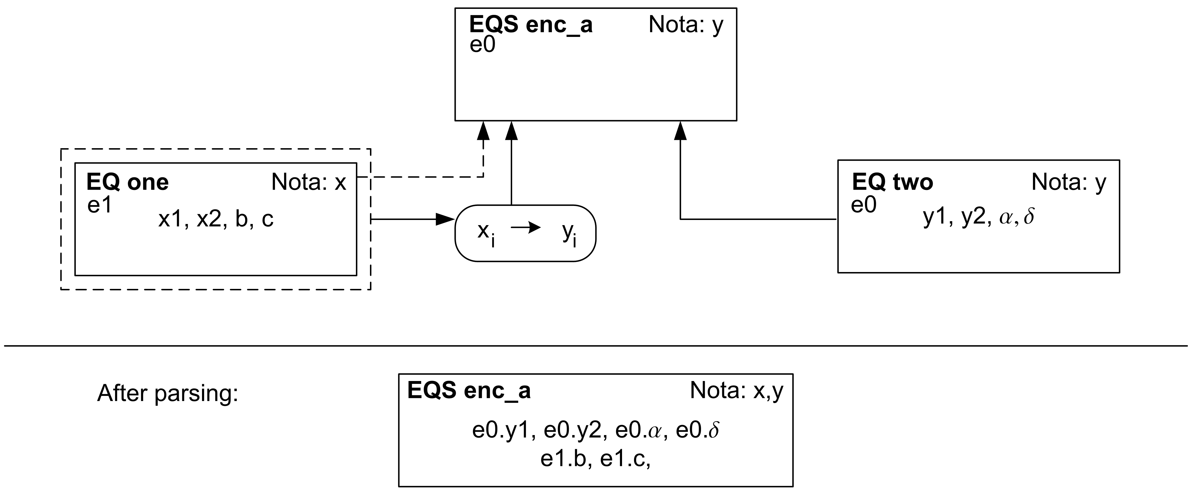
Figure 1: Visualization of the variable naming when using the connector. Note: this figure must be updated to match the variables and names used in this example.
Equation system
To construct the equation system, go to the Equation System tab and take the following steps.
- Load the user equation
- Click on “Add EQU/EQS”
- Add the user equation as usual
- Select and load the colleague’s equation, but do not confirm to close this popup window
- Make sure that the Naming policy is encapsulate
- Turn on the option Use connector und load your saved connector
- Confirm
- Your equation system should now contain the colleague’s equation, but with your connector in the Connector column
- Add the user equation in the usual way without specifying any connector
- Save the equation system
The equation system has ID 182753.
Evaluation / Simulation
Go to the “Simulation” section and do the following:
- Load your equation system in the tab Equation System
- Set the maximum Value NJ to 2 in the tab Indexing
- Go to the tab Specifications; you will notice that the variables
and
are part of the problem. In addition, the variables
- Assign the variables
- Assign the variables
and
as iteration values
Initialization and results
To initialize and specify the model, take the following steps:
- Initialize this example with the design values and initial guesses given in the previous examples
- Save the variable specification
- Save the simulation
- Go to the Evaluation tab and generate the code for your preferred environment
- Solve the system using the generated code
This simulation is available with ID 182754 with variable specification 182755. The solution will be the same as in the previous examples. This example shows that connectors can be much smaller if encapsulate is used because the remaining variables will be placed in their own namespaces and hence cannot be matched by accident.