Use of Ports and Streams III – Creating a Unit for Flowsheet Simulators

On this page

ChemCAD

The unit export to the User Added Module of Chemstations’ ChemCAD exists only as PDF thus far and can be obtained here. Currently, developing this feature further is not prioritized.

Aspen Plus

This example shows how to export self-implemented models from MOSAICmodeling via Aspen Custom Modeler (ACM) to Aspen Plus in order to take advantage of Aspen’s property functions and integrate customized unit operation models into a flowsheet. The following description can also be obtained as a PDF here.

Model description

We want to export the model of a mixer as unit from MOSAICmodeling. The model equations, which are based on the MESHI approach, are shown below:

$\begin{align*}&0 = F_{s=1} \cdot x_{s=1,c} + F_{s=2} \cdot x_{s=2,c} - F_{s=3} \cdot x_{s=3,c} \\[2ex]&0 = F_{s=1} \cdot h_{s=1} + F_{s=2} \cdot h_{s=2} - F_{s=3} \cdot h_{s=3} \\[2ex]&0 = \sum_{c=1}^{NC} x_{s=3,c} \\[2ex]&0 = P_{s=1} - P_{s=3} - \Delta P\end{align*}$

The model consists of the component mole balance and the energy balance. In addition, the mole fractions of the outlet must sum up to one. This equation is only formulated for the output because the inlet composition is usually determined by the user or by an upstream unit. Finally, the mixer can include a pressure drop.

Workflow within MOSAICmodeling

The first steps must be taken in MOSAICmodeling.

Engineering Units

The ACM export operates on engineering units. Therefore, you need to set up a set of engineering units in the Engineering Unit Set of the “Model” section:

Add the following units to your unit set, either by creating them yourself or by using the pre-defined units in our model library:
- bar
- °C
- m³ per kmol
- GJ/kmol
- kmol/h
- kmol/kmol
Save the unit set

The unit set is available with ID 182841.

Notation

Go to the Notation tab and add the following symbols to your notation:

Base names

$\Delta P$ , pressure drop
$\theta$ , temperature
$F$ , mole flow
$h$ , molar enthalpy
$P$ , Pressure
$v$ , molar volume
$x$ , mole fraction

Indices

$c$ , component index 1..NC
$s$ , stream index 1..NS

Proceed to the Engineering Units tab and then go to Unit Preassignment. Assign the following units to the variables specified below:

$\Delta P$ : bar
$\theta$ : °C
$F_s$ : kmol/h
$P$ : bar
$h_s$ : GJ/kmol
$v_s$ : m³/kmol
$x_{s,c}$ : kmol/kmol

Save the notation. This notation is available in MOSAICmodeling with ID 182835.

Interfaces

Interfaces are necessary

to embed the external function calls to calculate the molar enthalpy and
to connect ports to external elements.

The necessary steps to set them up are outlined below:

Go to the Interface tab and load the saved notation
Add a reasonable description
Go to the tab Interface Fields. Add the variables $h$ , $\theta$ , $P$ , and $x_c$ . Name them “ACM liquid molar enthalpy”, “ACM temperature”, “ACM pressure”, and “ACM liquid mole fraction”, respectively. All of them should be of Dim Scalar, except for $x_c$ . Specify $h$ as Out and the others as In. If the units do not appear automatically, assign the correct unit to the four variables
Go to the tab Pattern Assistance and select “Other”. Select ACM Calculate Molar Liquid Enthalpy in the combo box. The required fields will appear below under Fields of Specific Interface
Verify that all the required fields are set up correctly. In the column Specified, it should read “yes” for all variables
Save the interface
Click on “New” and load the stored notation again
Add a description
Go to the tab Interface Fields. Add the variables $h$ , $\theta$ , $P$ , $x_c$ , $v$ , and $F$ . Name them “ACM molar enthalpy”, “ACM temperature”, “ACM pressure”, “ACM overall mole fraction”, “ACM molar volume”, and “ACM total molar flow”, respectively. All of them should be of Dim Scalar, except for $x_c$ . Specify all variables as In/Out. If the units do not appear automatically, assign the correct unit to all variables
Go to the tab Pattern Assistance and select “Other”. Select ACM Stream Data in the combo box. The required fields will appear below under Fields of Specific Interface
Verify that all the required fields are set up correctly. In the column Specified, it should read “yes” for all variables
Save this second interface

The interfaces are available with IDs 182840 and 182842.

Function

Aspen Custom Modeler has many built-in functions (procedures), e.g., for enthalpy, density, viscosity, fugacity, activity coefficient, etc. These functions can be embedded in a MOSAICmodeling model and are generic function calls, The calculations will be performed according to the selected property package (NRTL, SRK, PENG-ROB, etc.) for every simulation. This allows easy model re-use.

In this example, the enthalpy of the liquid streams is calculated by an Aspen Custom Modeler procedure. As the enthalpy is a function of pressure, composition and temperature, the procedure has the following structure:

$h = \mathrm{ACMCalculateMolarLiquidEnthalpy} (\theta, P, x_c)$

in which $h$ is the liquid molar enthalpy in GJ/kmol, $\theta$ is temperature in °C, $P$ is pressure in bar, and $x_c$ is the mole fraction of component $c$ . Note that these units matter because ACM cannot know which units are being used in the MOSAICmodeling model. For this purpose, engineering units are included.

To set up the function call in MOSAICmodeling, go to the Function tab and do the following:

Add a reasonable description
Load the notation specified in this example
Click on the combo box below Interface Settings in the tab Interface & Body Settings and select Load interface. Load the previously created interface for the liquid enthalpy. Input and output variables should be filled automatically. Make sure that the correct engineering units are set for input and output variables
Save the function

The function has ID 182843.

Connectors

To be able to export the mixer as unit, we need to prepare the connectors for the port as well. Therefore, go to the Connector tab and do as follows:

Load the saved notation as both Sub and Super Notation
Set up the variables given in Table 1 in the Sub and Super Notation and select the correct units
Save the connector
Repeat these steps for the other two connectors

The connectors have the IDs 182845, 182846, and 182847.

Sub Notation	Super Notation (Inlet 1)	Super Notation (Inlet 2)	Super Notation (Outlet)	Unit
$\theta$	$\theta_{s=1}$	$\theta_{s=2}$	$\theta_{s=3}$	°C
$F$	$F_{s=1}$	$F_{s=3}$	$F_{s=3}$	kmol/h
$P$	$P_{s=1}$	$P_{s=2}$	$P_{s=3}$	bar
$h$	$h_{s=1}$	$h_{s=2}$	$h_{s=3}$	GJ/kmol
$v$	$v_{s=1}$	$v_{s=2}$	$v_{s=3}$	m³/kmol
$x_c$	$x_{s=1,c}$	$x_{s=2,c}$	$x_{s=3,c}$	kmol/kmol

Table 1: Connector variables and units for all three connectors.

Equation system

Go to the Equation System tab and take the following steps:

Load the notation you created for this example
Add a helpful description
Add the four equations you formulated above to the equation system
Go to the Functions tab and add the function you created above to the equation system. Add three applications ( $h_{s=1}$ , $h_{s=2}$ , and $h_{s=3}$ with their respective inputs)
Save the equation system. Note: it is not necessary to save the equation system first and then add this equation system again in combination with the ports as outlined below. We do this for clarity here. However, the ports could also be added directly to this system

Now, we will define an equation system for the unit. Hence, we will need ports. Ports are necessary to allow the model to be connected to streams. They consist of an interface containing the required variables for connectivity and one (or several) connectors translating the variable names from the model to the interface definition. For the mixer, two inlet ports and one outlet port is necessary.

To set up the unit, perform the following steps:

Click on “New” in the Equation System tab
Load the notation again and a description for the unit
Load the equation system you save above
Go to the tab Flowsheeting and then to the tab External Ports
Click on “+ Port”. Name the port “Inlet1”, load your interface for stream data and your connector for inlet 1. Click on “Check Port Configuration” and then confirm
Repeat the last step twice to add the second inlet and the outlet port. Remember to set the direction to “out” for the latter
Save the unit

The normal equation system has ID 182844 whereas the unit has ID 182848.

Code Generation

In the final step within MOSAICmodeling, we need to export the code to ACM. Therefore, proceed as follows:

Open the unit in the “Simulation” section
Add an appropriate description to the simulation
Set the maximum value of the component index $c$ to 2 and the maximum value of the stream index to 3. Click on “Confirm Index Data”.
Go to the Specifications tab and then to the Variables tab. The enthalpies of the three streams should be classified as calculated values.
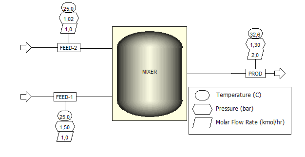
Assign all values from the inlet ports as design values. In addition, specify the molar volume of the output port as design value. This variable is not used in the model and is hence not calculated. It is only included because it is a requirement of the predefined interface.
Assign the remaining variables as iteration values.
Specify reasonable values and initial guesses for all variables. A possible initialization is given in Table 2.
In the tab Namespaces, you can give assign your own names for the namespaces. This is very important if many ports are used. Since the ACM stream interface is selected as the super notation, the namespaces are the only way to differentiate the variables.

Finally, go to the Evaluation tab and then select the Generation tab. Select ACM NLE Functions as Equations from the predefined language specifications and press “Generate Code”. The code in tab View Code is now ready to be copied and compiled in Aspen Custom Modeler. The simulation is stored with ID 182849 with variable specification 182850.

Name	Description	Value / Initial guess
$\Delta P$	Pressure drop in mixer in bar	0.0
$\theta$	Feed temperature in port 1 in °C	25.0
$\theta$	Feed temperature in port 2 in °C	25.0
$F$	Feed to port 1 in kmol/h	1.0
$F$	Feed to port 2 in kmol/h	1.0
$P$	Feed pressure in port 1 in bar	1.02
$P$	Feed pressure in port 2 in bar	1.02
$v$	Molar volume in port 1 in m³/kmol	0.0
$v$	Molar volume in port 2 in m³/kmol	0.0
$v$	Molar volume in port 3 in m³/kmol	0.0
$x_{c=1}$	Mole fraction of component 1 in port 1 in kmol/kmol	1.0
$x_{c=1}$	Mole fraction of component 2 in port 1 in kmol/kmol	0.0
$x_{c=2}$	Mole fraction of component 2 in port 1 in kmol/kmol	0.0
$x_{c=2}$	Mole fraction of component 2 in port 1 in kmol/kmol	1.0
$\theta$	Outlet temperature in °C	25.0
$F$	Outlet flow in kmol/h	2.0
$P$	Outlet pressure in bar	1.02
$x_{c=1}$	Mole fraction of component 1 at outlet	0.5
$x_{c=2}$	Mole fraction of component 2 at outlet	0.5

Table 2: Overview of parameter values, initial guesses, and the solution.

Workflow within Aspen Custom Modeler

Configuration of the component list

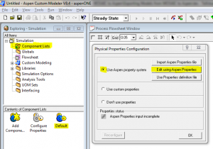
Open the ACM user interface. For this example we are using version 8.4. Before creating the model, it is necessary to configure a component list and a property package. In the Model Explorer select Component List and then double click on Default. Select the use Aspen property system option and click on Edit using Aspen Properties.

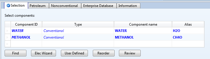
ACM_component_list — Figure 1: Configuring the Default Component List in ACM.

This will open the Aspen Properties user interface. Here the component list and property methods can be specified normally as when starting an Aspen Plus simulation. In order to verify the non-ideal enthalpy calculations, a binary mixture of water and methanol will be used. Add water and methanol to the component list.

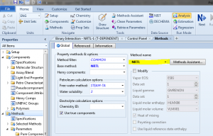
Aspen_Properties_List — Figure 2: Component List in Aspen Properties.

Click Next to go to the Methods tab and select NRTL as the main property method.

Aspen_Properties_Methods — Figure 3: Method Selection in Aspen Properties.

Click Next one more time to retrieve the binary interaction parameters and again to run the property analysis. Once this is completed successfully, close the Aspen Property window and save the file when asked.

Back to the ACM window, it should state that the Component List setup was completed. Click on OK and add the available components to the ACM component list.

Creation of new model

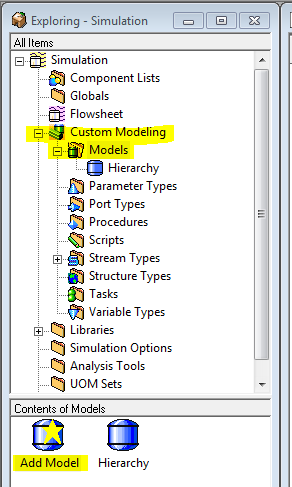
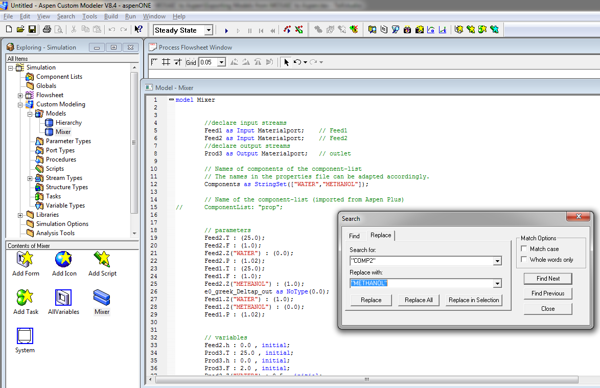
Now it is necessary to create a new model that will receive the code generated in MOSAICmodeling. Again on the Model Explorer palette, select Custom Modeling $\rightarrow$ Models and then Add Model as highlighted below.

ACM_models — Figure 4: Adding a New Model in ACM.

Name the model and paste the ACM code exported from MOSAICmodeling in the code window.

By default, the MOSAICmodeling code generation will:

- Name the model as mosaic_model

- Name the component list as prop

- Name components as COMP1, COMP2, etc.

- Name inlet ports as Feed1, Feed2, etc.

- Name outlet ports as Prod3, Prod4, etc.

The model name appearing on the code window must be the same as the name previously given, so change the fist line from mosaic_model to your given name. Comment by adding // or erase the line with the component list declaration to make ACM use the default component list as desired. It is essential to keep consistency in the component names, therefore the Component ID for water should be WATER and for methanol it should be METHANOL as previously defined. By using the tools search for and replace, it is possible to replace COMP1 and COMP2 by WATER and METHANOL.

One might also want to rename the ports to make it clear to the user where to connect the streams. In a distillation column, for example, it’s advisable to rename the outlet ports as Distillate and Bottom Product, rather than Prod2 and Prod3. This is not important for the mixer.

The default icon for all models generated in ACM is the flash vessel. It is possible to change this icon and design customized icons that reassemble the real equipment. Under the Contents of your model, there’s an option to Add Icon.

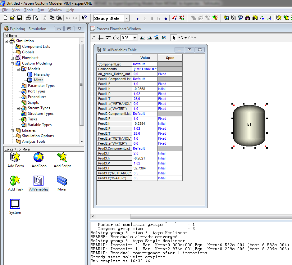
ACM_Mixer — Figure 5: Coding Window in ACM.

Once these minor modifications are done, right-click on the coding window and click on compile (sh. Compilation should be completed without any errors. Close the window containing the code. In the Model Explorer palette, click on the mixer model and drag it to the Process Flowsheet Window to add a mixer unit to the flowsheet.

A light-green square on the lower right part of the ACM window indicates that the degree of freedom is zero and the simulation is ready to be executed. It would show a red arrow pointing upwards if the model is overspecified and pointing downwards if it is underspecified. Run the model by clicking on the run button in the upper part of the screen. Check the results.

ACM_run — Figure 6: Flowsheet Simulation and Results.

Export of ACM model to Aspen Plus

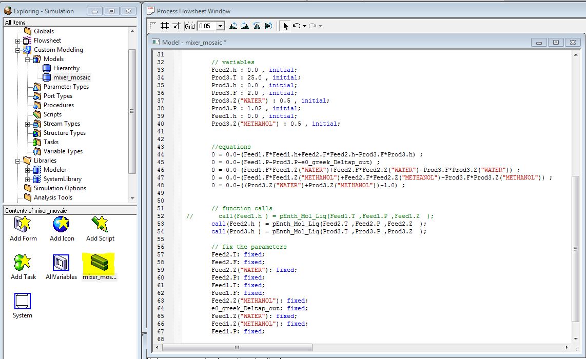
Now the model is to be exported to Aspen Plus. For this example we are using Aspen Plus version 8.6. When simulating a unit in an Aspen Plus flowsheet, the inlet ports will be connected to streams. Streams in Aspen Plus already have a built-in function to calculate the enthalpy once pressure, composition, and temperature are specified. This means that there is no need to calculate the enthalpy of the inlet stream using a function anymore. Therefore, these lines must be commented by adding // or deleted from the ACM code. This can be done in the Model Palette/Models then selecting the highlighted icon under contents.

code_window — Figure 7: Opening the code window for a model.

- ADD: HOW TO OPEN AND EDIT THE CODE. FEED info can be retained as initials

Depending on the installed version of Aspen, it may be necessary to have a proper version of Microsoft Visual Studio installed in order to export the model. It is possible to export to DLL, in order to generate a .dll file which can be read by Aspen Plus as a unit operation. It is also possible to export to MSI, which will generate an .msi file that can later be used to install the .dll file.

In the Model Explorer right click on the model name and select EXPORT TO MSI. When asked “Do you want to install the model now?” click yes and follow the installation steps. Keep the default location for the file.

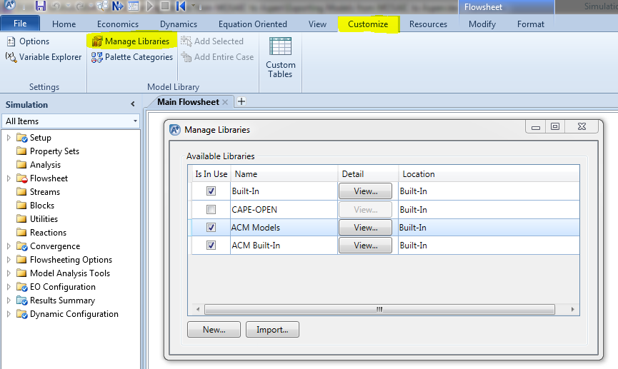
Once the file has been installed correctly, start a new Aspen Plus simulation file, select WATER and METHANOL as components and NRTL as property package. Run a property analysis and then enter the simulation environment. To enable the ACM models to be shown in the Model Palette, select the tab Customize and then Manage Libraries and then activate the ACM Models.

AspenPlus_enabling_ACM — Figure 8: Enabling ACM Models in the Model Palette.

Add the customized mixer model to the flowsheet and repeat the simulation done in ACM. The results should be the same.

AspenPlus_simulation — Figure 9: Simulating the Mixer.